Modeling Vehicle Handling in MATLAB

January 21, 2026

Throughout 2025 and 2026, I've been working extensively to research, design, and develop the steering system for UBC Solar's 4th-generation car. A large part of this has involved building up scripts for the UBC-Solar/vdx-simulation repository that allow us to model and optimize the unique characteristics of our atypical solar car steering/suspension systems.

# A Tire Model

Tire behaviour is notoriously empirical—and contrary to the open-source philosophy of computer science—most of the advanced research about tire performance is locked behind corporate doors. Yet, a reliable tire model is fundamental to any simulation of vehicle dynamics. As the sole physical interface between the car and driving surface, the tires "conduct" every aspect of the vehicle's handling response—making their accurate virtual representation perhaps the most critical part of a comprehensive dynamics simulation.

Thus, Pacejka's classic empirical Magic Formula was of little utility to the team, given the extensive physical testing required to derive its coefficients to produce an accurate tire model. Instead, the physical 3D Multi-Line Brush Tire model as proposed by Conte seemed to be a much less experiment-dependent approach that still produces highly accurate force and moment curves. The primary benefit of this model was its physics foundation—using accessible physical constants such as contact patch geometry, bristle stiffness, and friction limits—rather than being a curve fit of non-existent experimental data.

While our implementation of this model was slightly watered-down from the full range of dimensions in the original thesis, it still provided a solid foundation that allowed for the simulation of larger systems on the car.

Of importance for other simulations, we can use the following formula (derived for our unique tire geometry) to model tire slip as a function of lateral force:

\alpha = \operatorname{arccot} \left( \frac{2K}{FA} \int_{0}^{2a} (2a - x)b(x) \, dx \right); \quad b(x) = \sqrt{r^2 - \left( \sqrt{x^2 + \delta^2} - (R - r) \right)^2}

As I work to take this article out of its draft form I hope to share more about the fascinating math here.

# Asymmetric Thrust Energy Losses

Contrary to most automotive vehicles, solar cars often are one-wheel drive—driven by a single hub motor on one of the rear wheels. This forces the question—which rear wheel should be driven? For a solar car, the answer may seem trivial: whichever wheel makes the car more efficient. However, actually determining which wheel—port or starboard—results in less power consumption isn't so simple.

To start, I should actually clarify what the real difference is between each configuration, as it isn't really left/right at all. In fact, what we actually seek to explore is the impact of road crowning, and how efficiency compares when we power an uphill wheel as opposed to a downhill wheel.

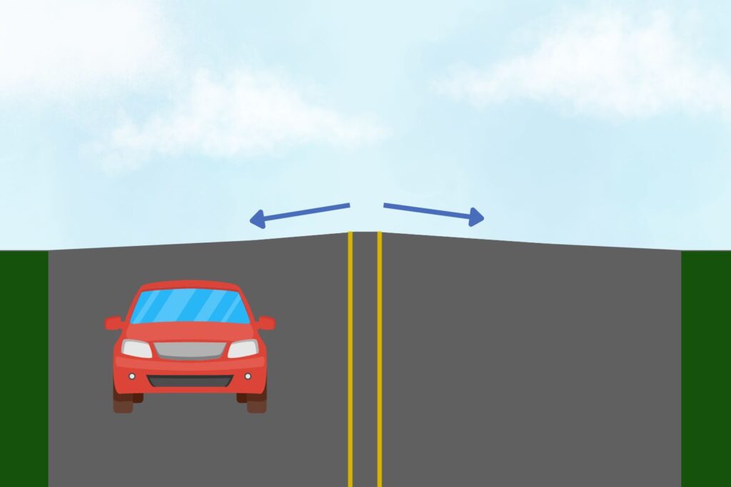
Diagram of road crowning — Typical Road Crowning (image from carparts.com)

As is standard in mechanical engineering, a free-body diagram is helpful for understanding the forces at play, leading me to create the following (relatively crude) model of what's going on:

The primary simplification in this model is taking the drag force to act at the CoM of the vehicle. Is this representative of reality? No. However, since $F_D$ is a highly complex function of the car's aeroshell, velocity, and crosswind, we opt to make this assumption and stay focused on the core dynamics at play.

Now, setting up equations to balance forces and utilizing the tire model to relate tire slip $\alpha$ to lateral force $Q$ , we get a nonlinear system that can be handed off to MATLAB to solve. Many iterations later, and we find that the equilibrium state (not sliding sideways off the road) looks like the following:

Driver steer magnitude:		     0.47°
Front wheel slip:		           0.70°
Rear wheel slip/Chassis tilt:	 0.23°

Some simple trigonometry and we can derive that

P_{loss}=Qv\sin(\alpha)

for each tire. Using this, we can estimate the power losses for a given configuration as follows:

Estimated Power losses @ 40 km/h:
	11.25 Watts

Comparing this value between port/starboard drive wheels for our given car geometry helped the team to understand the implications of each, ultimately leading to the decision being made to power the uphill wheel.

# Steering Linkage Geometry

Modeling the steering geometry for our car has been one of the most rewarding experiences I've had on Solar. In fact, this section probably deserves its own article in the future, where I hope to share more about some of the misnomers about steering that creep into many of the enthusiast articles you'll find on the topic.

For a primer on Ackermann steering geometry, I can recommend The Contact Patch which is the foundation for much of the analysis I performed.

If you gave that article a read, it likely won't come as much surprise that for our solar car, we pursued a six-bar rack-and-pinion steering linkage—primarily for its ability to better approximate the theoretical ideal of pure-rolling throughout steering travel. From a more mechanical side, this linkage was also a great fit for packaging on our car, and gave more freedom for designing around bump steer.

So, of what use is a kinematic model for steering? Simply put: I needed to choose dimensions and position of the steering arm, how far to set back rack/tie rod interface from the wheels, and what static inclination the tie rods should experience. Tweaking any one of these dimension cascades into a different Ackermann compliance curve, steering ratio, induced tire slip, and ultimately power efficiency. Without a computational model, I'd be blind to these trade-offs and would struggle to optimize the geometry in this large solution space. Creating a visualization (as shown below) gives me a tool to catch interference issues without leaving MATLAB, and understand the physical implications of the dimensions as I test them.

3D steering linkage visualization, straight

3D steering linkage visualization, steered

The mathematical core of this simulation treats the tie rod length constraint as a path intersection problem. For any rack position, the steering arm traces a circular arc about the kingpin axis while the tie rod enforces a fixed distance to the rack connection point. Solving for the angle $\theta$ that satisfies this constraint

\|\vec{P}_{\text{SA}}(\theta) - \vec{P}_{\text{ER}}\| = L_{TR}

allows me to extract wheel steer angles $\delta$ across the full steering range.

With wheel angles determined, I can evaluate and characterize the Ackermann compliance of a given geometry by tracking the distance between instant centres of the left and right wheels projected to the rear axle (IC distance). In this phase space, we would anticipate True Ackermann to produce zero IC distance throughout steering travel (both wheels turn around the same point). We can further describe three regions of this space: "pro-Ackermann", "anti-Ackermann", and "lazy Ackermann". As shown below, referring to a given geometry as simply "anti-Ackermann" (as is often applied to formula-style cars) or "pro-Ackermann" discards the nuance that a given geometry is represented by some curve in this phase space, not by simply a region a portion of it may lie within.

This same constraint-based solver can be utilized to plot all sorts of metrics that were also helpful in selecting steering geometry and understanding its implications.

Disclaimer: plots in the steering section of this post are not reflective of final geometry, and in fact, show quite poor geometry

This dynamic, interactive environment allowed for great design iteration, and gave me a confidence in the geometry we ultimately proceeded with for the fourth generation car. The extensive visuals made the process super intuitive and was super beneficial for keeping others on the team in the loop of what the geometry actually looked like as iterations progressed.

# Suspension Member Forces

While working on the simulation for our fourth-generation car, I was closely involved with the determination of our car's suspension geometry—and helped bring about the pullrod/bellcrank configuration that our suspension was designed around. That said, I didn't work on the computational model of this system, and the graphic below is the work of one of my talented teammates.

# What's Next

Every simulation I've described could use assorted improvements to some combination of code style, computational efficiency, and documentation. While a lull in design work for the car isn't close on the horizon, eventually I hope to return to these scripts and make them more accessible!